Introduction

Integral Field Spectroscopy (IFS) is the technique that allows to obtain the spectra of a more or less continuous region of the sky. The light coming from different positions in the sky is conducted and resampled in the spectrographs by several different techniques (lens arrays, fiber bundles, image slicers....). These different implementations have produced a set of instruments, which, sharing the basics of the technique, produce very different representations of the spectra in the detectors. These apparent diversity leaded to the creation of reduction techniques and/or packages for each individual instrument. Together with the inherent complexity of this technique, this has reduced the use of IFS for decades to a hand-full of specialists, mainly attached to an specific instrument.
IFS specialists have realized of this handicap (Walsh & Roth 2002), and started to produce standard techniques and tools valid for any integral field unit (IFU). In particular, the Euro3D RTN (Walsh & Roth 2002) has created a standard data format (Kissler-Patig et al. 2004), a coding platform (Pécontal-Rousset et al. 2004) and a visualization tool (Sánchez 2004), useful for any of the existing IFUs. All these tools are freely distributed to the community, and can be downloaded from the Euro3D webpage and the E3D webpage. Following this effort we have started to develop a reduction package for the reduction of any fiber-based IFU data, and in particular PMAS data.

Coding Platform and distribution

We coded the algorithm in Perl, using the Perl data language PDL, in order to speed-up the algorithm testing phase. It is our intention to translate all the algorithms to C, following the standards defined by the Euro3D RTN (see above). However, even in this phase R3D is fast enough to produce valuable science frames in reasonable time, and its speed is similar or even faster than similar packages coded in IDL, like P3d.
A major advantage of using Perl is that it is a freely distributed, platform independent, language, and therefore R3D can be installed under almost any architecture without a major effort and not cost. The instructions of how to download and install R3D can be found in its webpage, where we will keep updated the different versions.

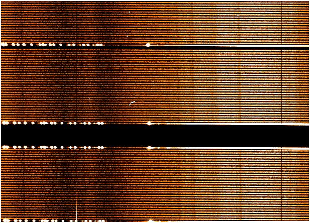Figure 1 Section of a raw frame taken with PPAK. It shows the spectra of a continuum-lamp in the science fibers and a ThAr spectra in the calibration ones.

IFS data reduction

In general terms any IFU raw frame looks quite similar. It shows several spectra spatially distributed through the detector following a certain pattern (Fig.1). Therefore, IFU data reduction share a similar sequence of steps independently of the instrument. We assume that the data has been BIAS corrected with whatever external tool, as an starting point for the reduction. Once BIAS corrected, the data reduction consist of: (a) identification of the positions of the spectra in the detector at a certain spectral pixel, (b) tracing of the peak of the spectra in the detector along the spectral pixels, (c) extraction of each individual spectrum, (d) distortion correction of the extracted spectra, (e) dispersion correction and (f) resampling in the sky position. Each of these reduction steps have been treated with a single (or a few) algorithm:

• Find the position of the spectra in the raw frame
  The location of the spectra in the central position of the CCD (or anyother defined by the user), can be found using the peak_find.pl script(Fig.2) . The output of this script is an ASCII file with the location of each spectra. It requires a continuum illuminated frame (whatever its origin).

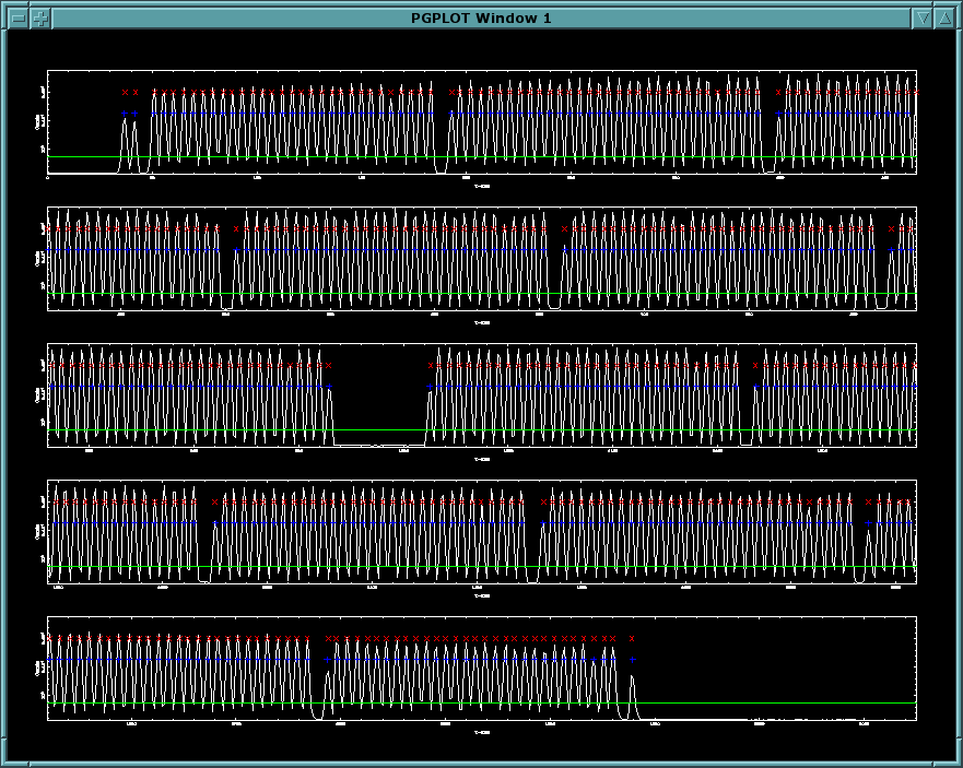  Figure 2 Example of the use of the peak_find.pl routine. It shows the identification of the spectra in a PPAK raw data.

• Trace the position of the spectra along the spectral direction
  Once located the spectra in the central position of the CCD, it is needed to trace this position along the spectral direction, using the trace_peaks_recursive.pl(Fig.3). This script requests the output of the previous one, and produce a FITS file (the trace) with the location of the spectra for each pixel in the spectral direction. It requires a continuum illuminated frame (like the previous one).

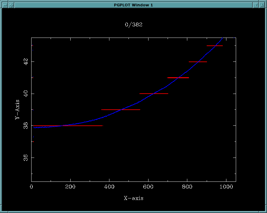  Figure 3 Example of the use of the trace_peaks_recursive.pl routine. Figure shows the distortion of the spectra along the CCD a PPAK raw data (blue line) showing the nearest pixel (red line).

• Extract the spectra
  Once located the spectra in the CCD it is possible to extract them, using the extract_aper.pl (for pure aperture extraction), or extract_aper_CT.pl (for Cross-talk corrected extraction, that is very slow)(Fig.4). It requires the trace frame, a raw-frame and the output is a FITS file with the length of the pixels in the spectral direction and the height the number of spectra.

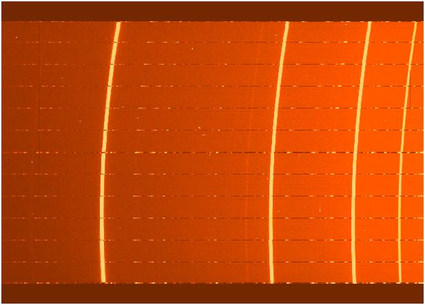  Figure 4 Example of the use of the extract_aper.pl routine. Figure shows a section of an aperture extracted spectra from a comparison ARC exposure taken with PPAK.

• Correct for the distortion & dispersion
  The distortion and dispersion corrections are handle in R3D separately. Using as input an ARC or an image with well defined emission lines, we perform a 1st order distortion correction, using the dist_cor.pl or dist_cor_cross.pl(Fig.5), identifying a single emission line. It produces as output a 1st-order distorted corrected frame and an ASCII file with the 1st order distortion corrections (*.dist.txt). Once performed this correction, it is possible to correct for second order distortion effects, using mdist_cor_sp.pl, identify several emission lines along the spectral dispersion direction. It produces as output a distorted corrected frame and a FITS file with the distortion correction solution (*.dist.fits).
  The distortion correction found using these scripts (*.dist.txt and *.disp.fits) can be applied to the science data using the mdist_cor_external.pl.
  The dispersion solution is found using the disp_cor.pl script, identifying the wavelength of several emission lines interactively. It produces as output a dispersion corrected frame and an ASCII file with the dispersion solution, that can be applied to the science data using the disp_cor_external.pl script.

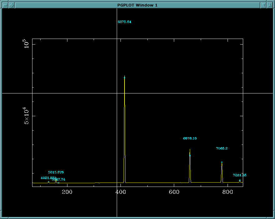  Figure 5 Example of the use of the disp_cor.pl routine. Figure shows the graphical tool for interactive identification of the ARCs emission lines.

• Fiber-to-fiber transmission correction
  Fibers have different transmissions that may depend on the wavelength. To determine the difference in the fiber-to-fiber transmission we use the fiber_flat.pl or fiber_flat_trans.pl scripts. They require a continuum illuminated frame as input frame, and produces a FITS file with the fiber-to-fiber transmission difference.
  The science frames can be corrected for this effect by dividing for this file, using the imarith.pl script.

Science Gallery

As we quoted before, R3D has been tested over different IFUs data, proved to be useful for reducing them in an homogeneous way. We present here a few examples of data reduced with this tool:

VIMOS DATA ON NGC 3242 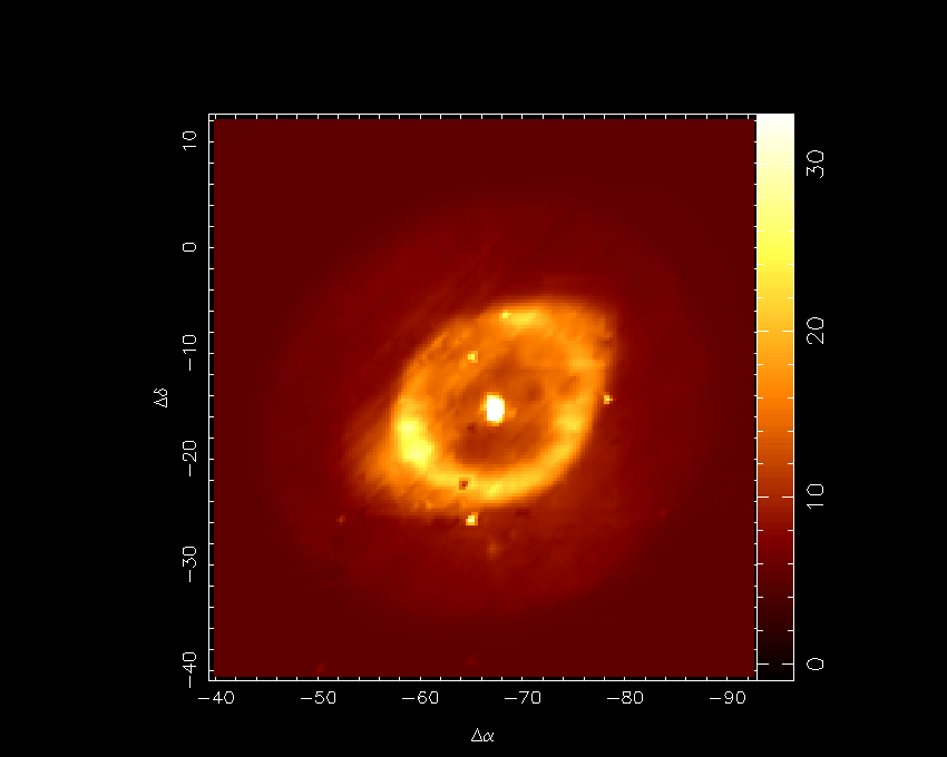Figure 6 Figure shows the planetary nebulea NGC 3242 observed with VIMOS in the Low-resolution blue mode (PIs: Schwartz & Corradi). It shows a cut centred in [OIII]5007, using E3D.

PMAS/Larr DATA: Bow-shock in Orion 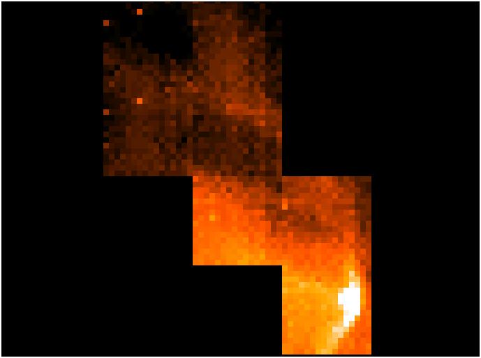Figure 7 Figure shows the Halpha emission in a Bow-shock in the Orion nebulae, observed with PMAS/Larr in the 1'' resoluton mode, performing a Mosaic. (PI: Angels Riera)

PMAS/PPAK DATA: Gas content in type I AGNs 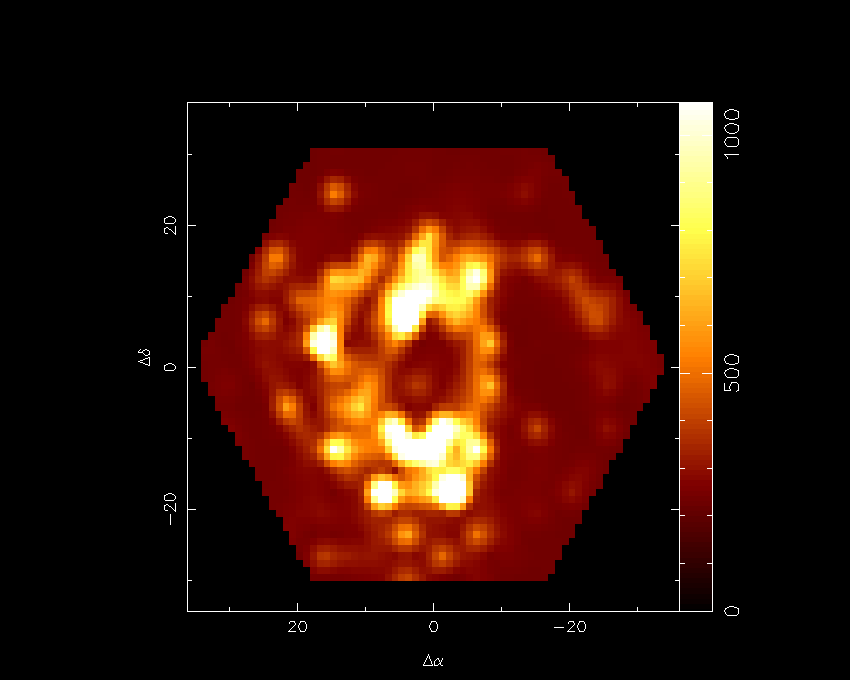Figure 8 Figure shows the continuum subtracted Halpha emission of a Seyfert 1 galaxy at z~0.03 observed with PPAK, using the V300 grating, covering the wavelegth range between 3700-7100 AA. (P.I., S.F.Sanchez)

PMAS/PPAK DATA: Stellar Populations in type I AGNs Figure 9 Figure shows a selected sample of spectra from the object shown in Fig. 8. It is shown the spectral range corresponding to Hbeta and [OIII], showing clear differences in the stellar populations in different regions.

Bibliography

• Arribas, S., Carter, D., Cavaller, L., et al., 1998, SPIE, 3355, 821
• Kelz, A., Verheijen, M., Roth, M.M., et al, 2005, PASP, submitted
• Kissler-Patig M., Copin Y., Ferruit P., 2004, AN, 159
• LeFevre, 0., Saisse, M., Mancini, D., et al., 2003, SPIE, 4841, 1670
• Pécontal-Rousset A., Copin, Y., Ferruit, P., 2004, AN, 325, 159
• Roth, M.M, Bauer, S., Dionies, F., et al., 2000, SPIE 4008, 277
• Sánchez S.F., 2004, AN, 325, 167
• Walsh, J.R., Roth, M.M., 2002, Messenger 109, 54