 Observer's Guide
Observer's Guide
This manual provides observing guidelines for MAGIC, the MPI für Astronomie General-Purpose Infrared Camera. It is not a comprehensive discussion of the techniques and tools of infrared astronomy. Rather, it provides a brief introduction to the problems associated with observing in the infrared and suggests general strategies for minimizing these difficulties. Separate documents contain detailed instructions for operating MAGIC itself.
The MAGIC team wants your observations to be successful. Please contact Peter Bizenberger (Tel. +49-6221/528311, FAX +49-6221/528246, e-mail: biz@mpia-hd.mpg.de) if you have any questions or suggestions.
THE MAGIC TEAM
       Name                       Specialty

Steven Beckwith      Science, Hardware
Peter Bizenberger    Hardware, Observer Support, Logistics
Christoph Birk       Software, Hardware
Tom Herbst           Optics, Spectroscopy, Science, Manuals
Stefan Hippler       Network Software, Sun Computer
Mark McCaughrean     Imaging, IRAF, Hardware, Science
Filippo Mannucci     Deep Imaging, Performance Spec's.
Grzegorz Pojmanski   Graphical User Interface, Software
Jürgen Wolf          Project Manager, Detector Spec's.
The main challenge of infrared astronomy arises from the enormously higher sky background levels in the IR compared with visible wavelengths, for example. The sky brightness in the V band is 22 mag / arcsec2 at a typical site such as Calar Alto. At 2 um, the sky brightness is approximately 13 mag / arcsec2 (measured with MAGIC on the 3.5 meter telescope). One normally wants to observe objects that are 8-9 magnitudes fainter than the sky level in the infrared, a challenge that visible wavelength astronomers rarely confront.
Infrared arrays differ from visible wavelength CCD's in requiring special semiconductors with a smaller energy difference between the valence and conduction bands. Typical materials include indium antimonide (InSb), platinum silicide (PtSi), and mercury cadmium telluride (HgCdTe). MAGIC's detector is a HgCdTe device.
The figure below contains a schematic drawing of the Rockwell NICMOS3 infrared array in MAGIC.
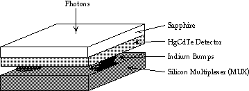
Figure 1
Photoelectrons are collected in the detector material and read out using a multiplexer. Because silicon multiplexer technology is much more mature, HgCdTe and InSb arrays are hybridized. This means that the detector material is cold welded to a silicon multiplexer using a series of small indium bumps. The actual HgCdTe detector material is grown on a sapphire substrate for mechanical strength. This hybrid arrangement has the benefit of lower crosstalk and less blooming and streaking compared with visible wavelength CCD's. Another significant advantage of the hybrid is that it permits non-destructive readouts of the detector, in which the voltage on the pixels can be measured without affecting charge collection. The main disadvantage is that the thermal mismatch between silicon and sapphire limits the size of these devices to approximately 10mm square.
The same noise sources that plague visible wavelength CCD's affect infrared detectors, although their relative importance can be quite different. The primary sources of noise in infrared observations are sky background, read noise, and dark current.
At wavelengths longward of 2.3 um, thermal emission from the atmosphere and telescope produces significant background. Shortward of 2.3 um, the sky signal is dominated by airglow emission from molecules, primarily OH and O2. This background can vary significantly, both spatially and temporally, (see Further Reading, below). Accurate photometry in the infrared means careful measurement of the sky level, and sky variations constrain integration times and general observing strategy.
Sky background introduces noise in two ways: (1) Imperfect subtraction of a varying sky level produces scatter in the photometry, and (2) Even in constant background conditions, there is shot noise associated with the high background photon flux. The latter noise is proportional to the square root of the number of background photons.
Each readout of the detector array has an associated noise level known as the read noise. This noise is a fixed quantity per readout, but it can be reduced with special sampling techniques to lower the effective read noise per integration (see below).
Current (1993) detector and multiplexer technologies have read noises of approximately 30 electrons per readout. Special sampling techniques can reduce this noise by a factor of approximately three. The next generation of arrays should produce less than 10 e- read noise per readout.
Dark current in an infrared detector results from the same process as in visible wavelength CCD's: thermal oscillations excite valence electrons into the conduction band, producing carriers in the absence of photon absorption. Since the band gap is smaller in an infrared sensitive semiconductor, IR arrays must be cooled to lower temperatures to suppress this dark current. MAGIC's detector and optics are cooled to approximately 77K with liquid nitrogen. The combination of LN2 cooling, smaller pixels, and improved detector materials means that MAGIC's dark current is negligible in almost all observing circumstances (measured at approximately 0.5 e- / sec).
The character of the noise sources described above gives a signal to noise ratio (S/N):
 (1)
(1)
where
t is the integration time (sec)
G is the photometric gain (e- / photon)
Fo is the total source flux (photons / second) from the target object
Npix is the number of pixels summed across the object
Ftot is the total flux (photons / sec) per pixel from the object, sky, telescope, etc.
Id is the dark current (e-/ sec)
RN is the read noise (e-)
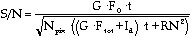
In most instances, the target object is fainter than the sky background. For a typical exposure with MAGIC using double-correlated sampling (see below), the read noise Nr is approximately 50 e-, and the dark current is 0.5 t e-. The photon noise associated with the sky background increases as the square root of time. Therefore, the signal to noise ratio increases approximately linearly with time until sufficient background photons have been collected to dominate the noise sources. This occurs when

i.e. when the background signal is more than the square of the read noise, or 2500 e-. With MAGIC, the conversion factor between electrons and Analog to Digital Counts (ADC - one ADC is the minimum signal unit recorded by the computer) in the image is 9.7 e-/ ADC. Therefore, any integration with less than approximately 250 sky counts is read noise limited , and the signal to noise ratio increases linearly with time. Longer exposures are background limited, and the signal to noise ratio increases only as the square root of time. The following figure shows this schematically.
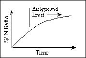
Figure 2
Integrating for much longer than the time needed to reach the background limit
does not provide any advantage to the observer, since a series of independent
exposures will also increase the S/N ratio as
 .
In fact, the variability of the sky level and other factors make it
advantageous to end an exposure when the background limit is reached. For
broadband images with MAGIC, this usually requires only a few seconds.
.
In fact, the variability of the sky level and other factors make it
advantageous to end an exposure when the background limit is reached. For
broadband images with MAGIC, this usually requires only a few seconds.
The MAGIC software does not require you to set up and take a large number of short exposures in order to observe near the background limit. There are options for automatically taking a series of images or adding a number of frames to a single file. There is a tradeoff between adequately sampling any sky variations and coming back from the observatory with tens of thousands of images. You should judge the best compromise based on the sky conditions, the required photometric accuracy, and your ability to record, transport, and reduce the resulting data. In our experience, exposure sequences lasting a minute or two work well (for example, fifteen frames of 4 seconds added together and saved to a single file). Single, longer duration exposures are fine for lower background observations with the narrow band filters or grisms.
We have ignored the photon shot noise associated with the target source in the discussion above, since the sky is usually considerably brighter than the object. In those lucky instances when the target is considerably brighter than the sky, the observer can achieve good signal to noise ratio very quickly, and the observing efficiency is then limited by telescope moves, exposure setup, etc.
The figure below is a schematic representation of the voltage on an individual pixel as a function of time. At the beginning of an exposure the voltage is set to a predetermined value by a reset. When the reset switch is opened, the voltage will jump to a variable new level* (the pedestal) and then increases linearly with time as charge from photoelectrons and dark current accumulates in the detector. This process continues until the detector is reset to the original level at the end of the integration. The linear behaviour of most modern detectors spans the range from zero charge to over 90% of the total capacity, which for MAGIC is approximately 300,000 electrons (30,000 counts).
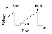 Figure 3
* The variability is caused by a quantum noise source called kTC noise, the thermally induced fluctuations of voltage on a capacitance C at temperature T.
MAGIC supports a number of detector readout modes suitable for various observing situations. These modes appear under the <Readout> menu and can be invoked with the ctype instruction from the command line interface and from macro files.
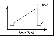 Figure 4
This is the simplest readout scheme. The pixels are reset and read out once at the end of the integration. This does not remove the variable pedestal level (kTC noise) and any initial offsets which can vary from pixel to pixel. We do not recommend using this mode for observation. Its main usefulness is in checking the signal level for saturation. Saturation occurs at 45,000 counts. (The previous page stated 30,000, but there is a 12,000 count offset in the software)
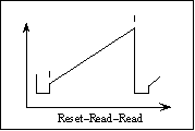 Figure 5
Also known as Double-Correlated Sampling, this is the most commonly used mode for general observing. The array is read immediately after the initial reset and before the final reset at the end of the integration. This eliminates the kTC noise and other offsets, but increases the read noise by [[radical]]2 because the noise from two readouts goes into a single image. We recommend this readout mode, particularly for broadband imaging where you reach the background
limit quickly (and can thus accept the higher read noise). Saturation occurs at 30,000 counts. Min. integration time = 60 msec.
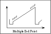 Figure 6
This variant of Double-Correlated Sampling is also known as Fowler sampling (see Fowler and Gatley 1990). The array is read multiple times after the initial reset and before the final reset (the values A and B tell MAGIC how many reads to perform). This scheme can reduce the read noise substantially, theoretically by a factor [[radical]]N. In practice, however, amplifier glow and other effects limit the reduction to a factor of approximately three with MAGIC. We recommended this mode in low background situations such as grism spectroscopy. Saturation occurs at 30,000 counts.
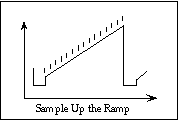 Figure 7
This readout scheme also reduces the effective read noise, since the pixel voltage is sampled N times at equal intervals during the integration. The total signal comes from a linear fit through the measurements (ctype ramp) or from saving the differences between adjacent reads (ctype speckle). The latter is used for speckle interferometry since the observer can save these adjacent differences as separate frames, each of which is a rapid exposure on the sky. Currently, MAGIC can take up to 256 frames at up to 20 Hz in this fashion. Warning: Be careful not to saturate the total signal in this mode. This can happen easily when observing lunar occultations, for example. You may have to settle for a shorter sequence. Saturation occurs at 30,000 counts total.
MAGIC calibration procedures, such as measuring the pixel to pixel gain variations using dome or sky flats, are similar to those used for visible wavelength CCD's. There are differences, however. For example, it is critically important to have frequent and accurate sky level measurements, since the sky is bright and variable at infrared wavelengths. On the other hand, the relatively short exposures, high backgrounds, and frequent sky measurements make dark current calibration unnecessary.
The measured detector voltage contains several contributions besides the source flux we wish to observe. We can write this voltage V0 as follows:
 (2)
(2)
where (as before)
t is the integration time
G(x,y) is the photometric gain measured in electrons/photon
at pixel location (x,y)
Fo is the number of photons/sec from the target object
Fb is the number of photons/sec from the sky background
Id is the dark current in electrons/sec
Here we explicitly recognize that the photometric gain can vary from pixel to pixel. We isolate the source flux by taking a sky frame whose signal Vs will be:
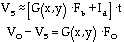 (3)
(3)
The difference between these voltages eliminates all undesired effects except the pixel to pixel gain variations. These can be calibrated with a flat field image (discussed fully below). The difference in signal between exposures of the dome wall with the lights on and off is:
 (4)
(4)
This is exactly the gain factor (times the constant Qt') remaining in equation (3) above. Division of equation (3) by equation (4) isolates the target object signal. Applying the same flat field to images of a known reference star eliminates Qt', giving the absolute flux calibration. As with CCD's, careful photometry requires frequent calibrator star measurements at a range of zenith angles.
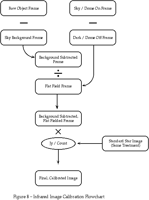
The flowchart on the next page shows the calibration steps discussed above.
Warning: Since the sky background can be significantly higher than the source flux, it is important to have an accurate measure of Fb. This means taking sky frames close in time to the object frames. Although it reduces observing efficiency, do not skimp on sky frames. You will regret it. There are macros in the data system to take frequent sky exposures with little impact on efficiency (see Moving Sky, below).
When the observing targets are pointlike or small, most of the array is, in fact, measuring the sky background level. A simple strategy to take advantage of this information is shown schematically in figure 9. Offsetting the telescope between exposures produces a sequence in which a subsection of the array contains the target object in one exposure and sky measurements in all the others. A median average of these sky frames will eliminate the pointlike sources (i.e. an image in which each pixel is replaced by the median of values at that location in all the sky frames) . Taking the median of, say, four neighbouring frames will give a sky level that is well-correlated temporally and spatially with that in the target exposure. This so-called "moving sky" frame works extremely well with virtually no penalty in observing time, since you should already be moving the telescope slightly between frames to account for bad pixels. You must move the telescope by at least twice the size of the largest observing target for this technique to be effective.
When the observing target is extended over a significant portion of the detector, the moving median will be contaminated by source flux and will not reflect the current sky level. In these circumstances, the observer must offset the telescope to a relatively
source-free area to measure the sky. A typical sequence may be Object-Sky-Sky-Object-Object-Sky-Sky... The atmospheric conditions are the major factor in deciding how frequently to measure the sky level. Note also that most "empty" fields contain numerous stars, particularly given the large field and high sensitivity of MAGIC. You should offset the telescope between sky exposures and form the median as before to eliminate point sources. The positive aspect of taking frequent off-source exposures is that it gives you an opportunity to monitor the atmospheric transparency, seeing, and focus using a star in the sky field.
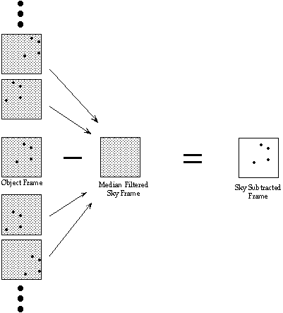
Figure 9 - Schematic Representation of the Moving Sky Technique
The flat field image provides a means of removing pixel to pixel gain variations in the array. There are several different techniques for producing the flat field, but they all share the goal of exposing the detector to uniform illumination. The image values in the resulting frame will be proportional to the pixel gains. Division of the object frames by the flat field will eliminate these variations.
Source-free sky exposures should contain only dark current and sky background flux, which is uniform over MAGIC's field of view. Subtracting an exposure of the same duration taken with the camera internally blanked off (a dark frame) will, in principle, yield an image of uniform illumination, in other words a flat field. In practice, however, the sky is almost never source-free, so we recommend the median averaging procedure (discussed above) to remove the stars. This type of flat field is like the moving sky frame, in that it comes without additional observing overhead - the same exposures can be used for object, sky, and flat. However, do not forget to take dark frames of the same duration to subtract dark current and other offsets if you use this type of flat field.
Two other caveats deserve mention. First, the flat field is divided into every exposure. Make sure the sky flat has sufficient signal to minimize additional noise. For this reason, sky flats are generally not practical for narrow band imaging. Second, the sky background may not be uniform spectrally. Sky flats are not recommended for grism spectra, since the bright emission lines will mimic higher detector gain. In the K band where thermal emission increases dramatically at the long wavelength end, the sky flat may reflect the gain variations at an effective wavelength quite different from the peak emission of your science objects. Proper calibration with a standard star of known spectral type should eliminate any difficulty, but extra care must be taken for high accuracy photometry.
Another way of obtaining uniform detector illumination is to point the telescope at a bright, blank surface. This produces a dome flat. At the 2.2 and 3.5 meter telescopes on Calar Alto, any bland part of the dome illuminated by lights will work. You will have to adjust the location, intensity, and direction of the lamps to get adequate signal levels without saturating the exposures. We have found that short integration times work well (i.e. 100 frames of 0.1 second averaged to a single file for K). Also check that no uneven shadows are cast on the part of the dome being measured.
Dark current and offsets appear in the dome flats as well, so we recommend taking an exposure of equal duration with the dome lights off. This also subtracts thermal emission of the dome in the K band and thus gives a flat field with the known intrinsic colour temperature of the lights.
The following are some general guidelines which will be appropriate for most observers:
1. Take flat fields in every camera and telescope observing configuration you use. This is extremely important. A K band flat will not suffice for J band observations, etc. Until we better understand the systematic characteristics of MAGIC, we also recommend taking flats in all readout modes you use (i.e. separate flats for Reset-Read-Read, Sample-Up-The-Ramp, Sub-arrays, etc.).
2. We have not observed variations in the flat field response within a single observing night. At this time, we recommend taking flats once per night. This can be done at any time - we routinely flat field just before or just after sunset. In good weather, the flat fielding measurements are often delayed until the end of the night.
3. We have not yet had enough photometric weather to cross check the sky and dome flat procedures. We therefore recommend taking dome flats as insurance, even if you plan to use sky flats. Please keep us informed of how well all these techniques work out.
The calibration procedures discussed above assume that the voltage on the detector is linearly proportional to the incident flux. We have measured this relationship for the detector in MAGIC. Figure 10 shows the number of counts per photon as a function of signal counts. The curve is normalized to 1 at zero counts. The deviation from linearity is less than 4 % at 30,000 counts. Normal reset-read-read exposures should not exceed 25,000 counts.*
Note that the linearity plot uses the median counts for the 65,536 detectors. Some pixels are more nonlinear and others less. Observers who need accurate photometry will want to correct all their exposures for nonlinearity before proceeding with the standard data reduction. We recommend using a second or third order polynomial fit to each detector's response. Speak to a MAGIC team member about getting the latest coefficients (these are essentially images whose individual pixel values are the response coefficients).
* This number can be lower for extremely bright objects (those which produce >20,000 counts in less than 0.5 second). This is due to charge accumulating in the detector between the reset and the first read (see the Readout Techniques section). Therefore, the difference between the first and second reads can be less than 25,000 with the total counts exceeding the linear range. In the extreme case, the detector saturates between the reset and the first read, and continues saturated until the second read. This produces almost zero total counts in reset-read-read mode. If you are in doubt, take a reset-read frame of the same duration and verify that the total counts are well below 45,000.
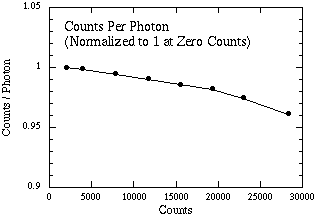 Figure 10
MAGIC has a spectroscopy mode which uses one of two direct-ruled ZnSe grisms in combination with the high resolution optics to give a double sampled spectral resolution of R=370 or R=185 (Herbst and Rayner 1993 - appended to this manual). One grism covers the entire K band in second order and the entire J band in fourth order. The second grism spans the H band in second order. The spectral resolution is defined by the focal plane slits, which are two and four pixels wide for R=370 and 185 respectively. Both the grisms and the focal plane slits are on motorized wheels, permitting the observer to switch rapidly (~30 seconds) between resolutions and between direct imaging and spectroscopy modes.
In addition there is a replica grism available.. This device gives a
spectral resolution of R=260 or R=130 for the two or four pixels wide slits respectivly.
This resolution means that the entire H
and K bands can fit on the detector simultaneously in first order. J band
measurements use second order. The replica grism can also be used with the
Spaltspinne for multi-object infrared spectroscopy. Contact Tom Herbst for more
details.
Spectroscopic observations with MAGIC are quite similar to direct imaging
measurements in most respects. For example, the observer must take sky and flat
field frames to remove background and pixel to pixel gain variations. On the
other hand, acquiring good spectra with MAGIC requires extra care and attention
to such things as persistence effects and telescope drift. The following
paragraphs explain how to use MAGIC in spectroscopy mode.
NOTE! Spectroscopy is only available with high-resolution optics execpt under special
circumstances (discuss with P. Bizenberger).
It is not possible to change grisms during night!
The easiest method for placing the target object in the slit is to take a sequence of direct images and use the telescope guide paddle or the user interface to place the object at the correct location. The slits in MAGIC are oriented along the y direction of the detector array (north-south if the Cassegrain flange rotator is at zero degrees). You can find the slit location in a ~5 second sky exposure with the slit and K filter. The slit wheel position is repeatable to approximately one pixel. We recommend that you check the slit position regularly, particularly in the higher resolution (narrower slit) configuration. Image persistence can be troublesome under low background conditions such as spectroscopy. To avoid problems, place bright objects in the correct detector column then move the source up or down the slit after inserting the slit and grism.
Exposures can be read noise limited at these spectral resolutions. To maximize observing efficiency, aim for at least 5000 electrons or 500 source counts per pixel in each exposure. As with direct imaging, there will be a tradeoff between fewer long exposures (sky variations and telescope drift) and many short ones (unwieldy number of frames).
Sky frames are important to remove airglow lines and thermal emission in the K band. For pointlike sources, the moving sky technique works well (see previous section). The displacements between consecutive frames must be along the slit direction, of course. For extended objects, move to a nearby blank sky location. Depending on how well the telescope offsets and returns, you may have to recenter the object in the slit. The autoguider can be a great help for these observations.
We recommend dome flats for calibrating the pixel to pixel gain variations, since only the longest sky exposures will have sufficient signal. The mounting flange contains an argon discharge lamp for wavelength calibration. In practice this lamp is rarely needed, since most frames will contain bright airglow lines whose wavelengths are well known (see Origlia and Oliva 1992 - appended to this manual).
The infrared spectral bandpasses contain numerous telluric absorption features. These can be removed by dividing each spectrum by that of a calibrator star. Consult a list of spectroscopic standards to determine the best spectral type for your program. All spectroscopic data reduction packages offer routines for interpolating across calibrator star absorption features to prevent artifact emission lines in the final spectrum. Also, dividing by a stellar spectrum introduces a spurious sloping baseline. This can be removed by subsequent multiplication by a blackbody of the same effective temperature as the calibrator.
In our experience, the standard astronomical data reduction packages such as IRAF or MIDAS contain all the tools necessary for extracting useful spectra from MAGIC frames. The documentation for these programs also contains useful information on difficulties associated with two dimensional spectroscopy, such as the extraction of tilted spectra and the removal of airglow lines.
First time users may appreciate an example of how a typical night of observing may proceed. The following (fictional) chronology assumes normal imaging operation at one of the Calar Alto telescopes.
TIME        EVENT

20:00       It is summer, so there is still approximately an hour until
            sunset. You arrive at the dome early to check the camera and
            to measure flat fields.
20:10       The MAGIC software is started and everything functions. You
            create a directory for the night's data files then move the
            telescope to the flat field position. Don't forget to take
            lamp-off exposures and to check for saturation in the flats.
            Take flat field images for all anticipated filters and
            readout schemes.
20:45       The sun is going down,  so you can open the dome to cool
            things off and look for a standard star.
21:00       You  select a standard star near the zenith. Focus the
            telescope for best image quality and when it is dark , take
            some photometric calibration images. Check the star counts
            (see below) to verify proper camera setup and good sky
            conditions. Some people find it easier to focus with many
            objects in the field, so you may want to use a globular
            cluster first. Look in the Astronomical Almanac.
21:20       The calibrations are complete and you begin observing your
            first program object. You move the telescope between
            subsequent exposures to account for bad pixels. The
            neighbouring frames can be used for the sky background and
            flat field, provided that your objects are point-like. Note
            that you need high sky levels to use the median averaged
            frame as a flat field.
22:00       Your first object is complete and you decide to observe a
            standard star at similar airmass. You will follow this star
            as it sets in order to get the extinction correction.
22:10 -     You continue observing program objects and standards.
5:00        Scattered sunlight is much less problematic at longer
            wavelengths, so you can observe much later than at visible
            wavelengths. Remember to monitor the focus, particularly if
            you are observing extended objects.
5:40        The sky is finally too bright to do meaningful observations
            (the detector saturates on the background in very short
            integrations). You decide to finish up with a last standard
            star. Checking the observing log, you notice that you
            observed one object in a filter for which there is no flat
            field image. You take the final flat and shut down the
            camera software.
6:00        The telescope is parked, the dome is closed, and you have
            filled out the log sheet for the evening. You start a backup
            of the night's data onto a DAT tape, switch off the camera
            electronics, and head down to the hotel for breakfast and
            sleep.
1. Switch on all three electronic boxes (two on the telescope, one in the control room).
2. Switch on the telescope. There is a separate manual for this procedure.
At the 3.5m telescope, the offset system must be in [[Delta]]alpha,[[Delta]]delta!
3. If you are at the 3.5m telescope, start the DACS program HEL NICA35/
Wait for the prompt and follow the instructions (i.e. type SETUP).
If there are any problems, logout
from the Magic account and try again to start the DACS program.
4. Login as magic22 at the 2.2m telescope or magic35 at the 3.5m
telescope.
Password: _____ (the current password will given to you by the night assistant
and will also pinned up in the control room)
5. Call up the GUI by typing MAGIC in the openwindow system.
You should check that the filter wheels are really rotating and that they stop again.
NOTE:
- Take care that you use the correct set-up.
We recommend checking the signal from a standard star at the beginning of each night's observing. This not only verifies that the camera is mounted, aligned, and operating properly, but also gives you some indication of the sky conditions. The procedure is quite simple:
1. Take a broad band exposure of a standard star of known brightness, for instance a K image of one of the objects listed in Elias et al. (appended to this manual and available in the GUI).
2. Measure the total counts on the star using the image viewer tools. Make sure the radius is set large enough to get all the starlight. Also measure the sky counts in a nearby region of the same size, or preferably in the same region in a subsequent frame.
3. Calculate the Counts for Zero Magnitude (CFZM) per second according to the formula:
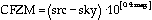
where src and sky refer to the counts per second on the star and sky, respectively. The value mag is the magnitude of the standard in the wavelength band being used. This calculation tells you how many counts that star would have produced if it were a zero magnitude object with a 1 second exposure.
4. Compare the CFZM with the table below. If you get a lower value which cannot be explained by poor sky conditions, there may be an alignment or setup problem. Call the night assistant or other qualified person to check that everything is working. You can check the alignment yourself. The procedure is described in the next section.
Table 1 - Counts for Zero Magnitude for Various Configurations*
Telescope, Camera Config               arsec per   J 108s-1   H 108 s-1  K 108 s-1  K' 108
                                         pixel                                      s-1
3.5m f/10 Wide Field Optics              0.81        8.17                           5.11
3.5m f/10 High Res. Optics               0.33

3.5m f/45 Wide Field Optics              0.18
3.5m f/45 High Res. Optics               0.07

2.2m f/8 Wide Field Optics                1.6
2.2m f/8 High Res. Optics                0.67
*Limited measurements at this time. Please contact your MAGIC support person for
updates
NOTE: MAGIC should be aligned properly when you arrive at the telescope. However, you should check at the beginning of every telescope run to be sure, and you may choose to align it yourself if it is out of adjustment.
MAGIC must be aligned on the telescope so that an image of the telescope pupil falls on an internal cold stop, called the Lyot Stop. The entrance pupil of the telescope is the primary mirror, an image of which is formed by the secondary mirror at a location a few centimeters beyond the secondary. For the purposes of alignment, we can consider the pupil to be the secondary mirror.
The collimator lens within MAGIC forms the image of the pupil/secondary at the location of the Lyot stop. This stop is a small hole mounted on a motorized wheel between the two filter wheels. If MAGIC is not properly aligned, the pupil image does not fall exactly on the Lyot stop and light is lost. By slightly altering the mounting angle of the camera (or perhaps rotating the Lyot stop wheel a small amount), the pupil image can be centered on the Lyot stop (see figure, next page).
It may be useful to think in terms of the complementary optical principle: the collimator lens projects an image of the Lyot stop at the distance of the secondary mirror. This image is the same size as the secondary mirror, and the purpose of the alignment is to make this projected image coincident with the secondary.
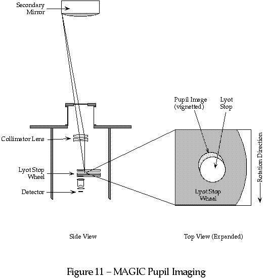
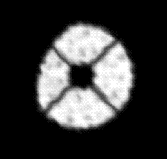 Figure 12 - Misaligned Pupil Image
NOTE: You must be looking at a star near the zenith to do this. You must have the appropriate Allen wrench and a ladder to adjust the mount. Do NOT use the lifting platform at the 3.5 meter, since raising the floor will shut down the telescope.
There are four sets of tipping screws on the camera mount. Each set has two holding screws and one pushing screw. The following figure shows the arrangement:
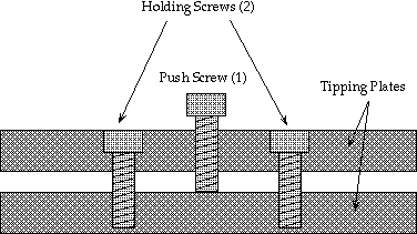 Figure 13
The camera must be hanging from the holding screws for the alignment procedure. Loosen the eight holding screws approximately two full turns. NEVER loosen these screws so that the gap between the tipping plates exceeds 5 mm, since the camera can fall off the telescope.
Tip the camera slightly by tightening one of the holding screws and take another (out of focus) image. If the alignment improves, keep adjusting that screw until the image is symmetric in one direction. If the alignment worsens, loosen that screw and, if necessary, tighten the opposite one. When you are satisfied with one direction, adjust the orthogonal pair of screws. Continue until the out of focus image is round and symmetric. The exact adjustment is not particularly critical. With experience, the whole procedure takes approximately 10 minutes.
When you are happy with the alignment, tighten all the push screws so that they are in firm contact with the other tipping plate. When all the push screws are in contact, they will define the plane for the tipping plate. Tighten all the holding bolts with the Allen wrench until they are quite snug. Tight holding bolts prevents misalignment as the telescope moves around the sky.
You should record the tipping in the MAGIC log book:
Example log entry:
29 Oct 1993, T.M. Herbst
Tipped up Blue MAGIC with High Res Optics on 3.5m f/10.
Tipping: 1mm gap in north, 1.5 mm gap in west, 0.5 mm in south, 0.0 mm in east.0
- Quit the GUI
- Change to the $home/tmp directory and delete all files with the extension *.pid and the file called shmsocket.
- Logout from the magic22 or magic35 account.
- Login again and type ctrl C before the openwin system starts up.
- Type px and kill all processes except tcsh, ps and more.
- Logout and switch off the three electronic boxes.
- Wait 30 seconds.
- Switch the electronic boxes on again, login and start up the GUI.
Not all filters are in MAGIC at once. We guarantee that the filters
marked with a ! symbol will be available. Please contact Peter Bizenberger
for special requests and to ensure that the filters you would like to use are
in the camera.
All wavelengths in um @77K, except those marked with *. These are measured at
room temperature.
NB1.500 50nm (3.3%) NH3
NB1.580 10nm (0.6%) cont.
NB1.700 50nm (3%) CH4
NB2.300 200nm (8.7%) CH4
You can create your own object list in the following format:
Object name | Alpha | Delta | Equinox | pm.A | pm.D | mag | Comment
Example:
HD 225023| 0:00:11.8| 35:32:14.0|1950|0.0000|-0.004|6.96|J=7.97
G158-27| 0:04:12.0|-7:47:54.0|1950|-0.056|-1.85|7.43|J=9.31
HD 1160| 0:13:23.1| 3:58:24.0|1950|0.006|-0.013|7.04|J=7.06
HD 3029| 0:31:02.3| 20:09:30.0|1950|-0.0001|0.011|7.09|J=7.25
Gl 105.5| 2:38:07.6| 0:58:57.0|1950|*|*|*|*
HD 18881| 3:00:20.5| 38:12:53.0|1950|0.0001|-0.030|7.14|J=7.12
G77-31| 3:10:40.5| 4:35:12.0|1950|0.112|0.15|7.84|J=8.74
HD 22686| 3:36:18.7| 2:36:07.0|1950|0.0017|-0.010|7.19|J=7.20
HD 40335| 5:55:37.6| 1:51:09.0|1950|-0.0005|-0.018|6.45|J=6.54
HD 44612| 6:21:09.7| 43:34:35.0|1950|*|*|*|*
Note! The line | character is used as a separator between fields.
If you don't want to put in numbers in some fields, you still have to use a
* character as a place holder.
You can prepare macro files in advance (see Macro Commands).
The following example shows a simple macro that moves a star to five positions
on the detector, starts a read at each and saves the data.
Example:
read ; start the 1. read
sync ; wait until the read is finished
tele rel 25 25 ; move the telescope
save -i -f 2 ; save the data as integrated starting from the second frame
sync ; wait until move and save is finished
read ; start the 2. read
sync
tele rel -50 0
save -i -f 2
sync
read
sync
tele rel 0 -50
save -i -f 2
sync
read
sync
tele rel 50 0
save -i -f 2
sync
read
sync
tele rel -25 25
save -i -f 2
sync
All files including a macro should have the extension:*.mac
Herbst, T. M. and Rayner J. T. 1993, in "Infrared Astronomy with Arrays: The Next Generation", I. S. McLean, editor (Dordrecht: Kluwer Academic Publishers), page 515 (Appended to this manual).