The wavefront measuring portion of the Wavefront Measurement Tool is a Hartmann style sensor. The optical test technique that is known as the Hartmann test was developed for the measurement of large telescope optics. In the test's original implementation, a mask equal in size to the optic under test was fabricated and placed on the optic. This mask had a number of small apertures distributed over its surface. The mirror/mask combination was illuminated from the center of curvature and the location of the ray bundle crossings near the focal plane recorded. These ray crossings may be analyzed to determine the local gradients of the mirror at the positions of the apertures in the mask. It is thus a geometric sort of measurement as opposed to an interferometric measurement. It is therefore free of some of the constraints of interferometry such as near monochromatic operation. As will be described below, in the Self-Aligning Hartmann sensor even greater flexibility is achieved through the use of sophisticated control and processing algorithms. First, we will describe the Hartmann technique as implemented in typical Hartmann wavefront measurement systems. Next, the specifics of the Self-Aligning system are presented.
One general drawback of the Classical Hartmann test is the need for the mask that is specific to the optic under test. Especially for large optics, these masks can be very expensive articles. In the AOA system, the mask is replaced by an array of lenses placed in a plane optically conjugate to the optic under test. These lens arrays thus may be small and inexpensive to fabricate. All that is required is that an image of the pupil of the optic under test be relayed onto the lens array. This assures that the individual lenslets map accurately onto the pupil of the optic and also that the wavefront at the lens array is identical (except for a radial scale change) to that at the optic.
There is another very important advantage to be derived from the use of a lens array in place of the mask. To see this it is easiest to consider that the mask is equivalent to a lens array equal in size to the optic under test and whose lenslets have a focal length roughly equal to the radius of curvature of that optic. There is no flexibility in this case since the focal length is set by the optic under test itself. In the case of a lens array conjugate to the optic under test, the focal length of the lenslets may be adjusted independently of the focal length of the optic under test. This allows an adjustment of the gradient measurement sensitivity of the sensor to suit the shape of the optic. It is this flexibility that makes it possible for the same sensor system to measure with very high accuracy the wavefront produced by a Hubble Space Telescope simulator and, with a change of lens array, the shape of f/0.7 paraboloids.
There is also a side benefit to the use of beam reduction optics before the Hartmann lens array. As the beam size is reduced the angular spread of the beam is magnified. This magnification increases the size of the gradients or tilts of the ray bundles from micro-radians to milliradians for typical testing configurations. Measurements of such large angles is not so prone to error due to mechanical and thermal instabilities in the sensor equipment as are interferometric sensors where dimensional stability must always be measured in parts of a micron.
In the earlier generations of Hartmann sensors several assumptions were made regarding the mapping of the sensor subapertures to the pupil of the system under test (the DM in this case) and the positioning of the lenslets with respect to the sensor focal plane. Both of these "alignments" were considered to be fixed in time. Thus, the mapping of the lenslet defined subapertures was determined once ("by hand") and used forever more. This mapping is critical to the successful measurement of the absolute wavefront or to the operation of a closed-loop correction system. Errors in the assumed placement of the subapertures are directly related to the absolute wavefront measurement error. The alignment of the lenslets to the focal plane determines where the Hartmann spots will appear on that focal plane. In earlier sensors that alignment was rigidly defined. That is, there was a predefined region of the focal plane that were used to determine the centroid of the Hartmann spot for a given lenslet. If the spot moved outside of that region, the dynamic range of the sensor was exceeded and the wavefront measurement became erroneous.
In the hbar sensor both of these limitations have been removed. Using thoroughly tested algorithms, the sensor determines the mapping of the lenslet defined subapertures to the pupil of the optic under test. This may be done as frequently as is required by the opto-mechanical stability of the system. Determination of this mapping is made possible by the ability of the sensor to shift from Hartmann spot imaging to pupil imaging under direction of the wavefront processor. Physically, this is accomplished by moving the detector/relay lens assembly longitudinally with respect to the lens array. Thus it may be made to relay an image of the lens array and system pupil image or of the Hartmann spots onto the detector. The analysis of the image of the pupil of the system under test superimposed on the lens array allows both the determination of the mapping of those lenslets onto the pupil and the shape of the pupil (e.g. central obscuration and/or spiders).
Further flexibility in the sensor is introduced by eliminating the rigid definition of the detector subapertures related to the lenslet subapertures. Once the pupil mapping is measured, the sensor re-configures itself to image the Hartmann spot pattern. This image is passed through algorithms that search for the Hartmann spots and define the detector subapertures around them. This greatly simplifies the mechanical alignment of the sensor. For example, if the sensor is placed so that its optical axis is not co-linear with the axis of the system under test a full aperture tilt is introduced. This makes itself evident in a general shift of the Hartmann spots with respect to the detector. In previous sensors, this full aperture tilt had to be kept within the dynamic range of the sensor. Using these more sophisticated algorithms, the sensor "realigns" its optical axis to that of the system under test.
Since neither of these algorithms requires much processing time, they may be repeated at any time that a shift in the optical alignment might be suspected. In the normal operation of the sensor, the self-alignment procedure would be executed at the start of each measurement set.
The tracker is a copy of the CHARM system developed by MPIA. It is essentially a centroid tracker that uses a sub-frame portion of a standard CCD camera to achieve frame rates up to a few hundred Hz.
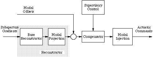
The purpose of this section is to define the logical organization of the MPIA deformable mirror (DM) control system. In closed-loop operation, the DM control system takes the subaperture tilts produced by the wavefront sensor and desired modal shapes supplied by the adaptive optics system, and produces actuator commands that are added to the flat voltages and applied to the DM. The logical organization of the control system is discussed in Section 2. The interface to the compensator code is presented in Section 3.
The logical architecture is shown in FIGURE 2.1. The subaperture tilts produced by the wavefront sensor are sent to the reconstructor. The reconstructor produces measured modal coefficients by two logical multiplications: a base reconstructor multiplication to produce OPDs, and a modal projection to produce the measured modal coefficients. The measured modal coefficients are subtracted from the modal offset signal and then filtered by the dynamic compensator to produce the compensated modal coefficients. The compensated modal coefficients are then multiplied by the modal injection matrix to produce the actuator commands. The supervisory control provides commands that open, close and reset the control loop, and that modify the parameters of the compensation algorithm. The following sections discuss each component individually.
FIGURE 2.1 Logical architecture of the DM control system.
The base reconstructor produces OPDs from the subaperture tilts produced by the wavefront sensor. The base reconstruction is simply a matrix multiplication, with the matrix determined by the solution of a least-squares problem.
The modal projection maps the OPDs produced by the base reconstructor into modal coefficients of modes selected by the user. Each column of the modal projection matrix will be the representation of a spatial mode in OPD coordinates. The modal representations will be selected to be orthonormal.
The full reconstructor is a single matrix multiplication that computes the measured modal coefficients from the subaperture tilts. The modes whose coefficients are to be determined are selected by the user at the beginning of operation of the DM control system. The full reconstruction matrix for the selected mode set can be determined in either of two ways. In the first method, the full reconstruction matrix is determined as a solution of a least squares problem that matches the observed subaperture tilts. The second method computes the full reconstruction matrix by multiplying the modal projection matrix for the selected mode set with the base reconstructor.
The actuator command voltages are computed by multiplying the compensated modal coefficients by the modal injection matrix. Each column of the modal injection matrix is the set of actuator voltages that are applied to the DM to produce the corresponding mode shape in a reflected wavefront.
The compensator filters the modal coefficients to provide compensated modal coefficients. Each modal coefficient uses the same compensation algorithm. The compensation algorithm provides proportional-integral (PI) control plus optional filtering of up to 3rd order. The algorithm is defined by the following transfer function:
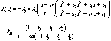 (1)
(1)
where kn is a normalization constant and:
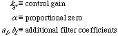 (2)
(2)
The controller parameters can only be adjusted in the set mode (see Section ).
At any point in time, the control code will operate in one of three modes: the set mode, the run/open loop mode, or the run/closed loop mode. Selection of a particular mode is controlled by the values of two logical variables, set and open. If the variable set is true, the control system operates in set mode. The variable open is not allowed to be false in this case, and will be set by the control code to true. If the variable set is false and the variable open is true, the control system operates in run/open loop mode. If the variable set is false and the variable open is false, the control system operates in run/closed loop mode.
In set mode, the control code simply waits to transition to one of the run modes. The DM control signal is set to zero. All initialization is done the first time the operational mode is entered. Upon transition to the set mode from the run/open loop or run/closed loop mode, all control states are set to zero, and the logical variable open is set to true.
In run/open loop mode, the control signal is held at its previous value. The filter states are updated normally, but the integrator state is set to hold the control constant.
In run/closed loop mode, all control states are updated and the control signal is computed by the compensation algorithm (see Section ).
The supervisory control provides the interface between the remainder of the adaptive optics system and the DM controller. It governs the transitions between control modes, and supplies the controller parameters needed to completely define the control algorithm. At each sample period, the supervisory control provides the commands the determine the mode switches (values for the control mode variables set and open). Control system parameters are also supplied when the controller is in the set mode. The parameters that can be specified are the number of spatial modes to be compensated Nm and the controller parameters . These parameters can be changed only during set mode - any changes made during either of the run modes will be ignored.
The compensator code must be invoked once each sample period. When invoked, the code is given access to the control system parameters, the control mode variables set and run, a pointer to the measured modal coefficients, a pointer to the modal offset signal, a pointer to storage where the compensated measured coefficients are to be placed, and a pointer to permanent storage that can be used to keep track of the internal controller states. The measured modal coefficients, the modal offset vector, and the compensated modal coefficients should each be double precision arrays of length Nm.
This section will be supplied as an addendum.